Introduction
A few months ago, Optiver launched a quite interesting Kaggle competition. Briefly, the goal is to predict the realized volatility during the next ten minutes for several stocks. To this end, you are given certain information about the order and trade book of each stock for the ten minutes window right before the target period. In this post, I will describe an approach that is different from the ones addressed in the discussion section (which by the way, warmly recommend to check).
A minimal background
Let’s say we observe the price \(S_t\) of an action for times \(t = 0, 1, \dots, n\). The realized volatility \(RV\) during this period is defined as the square root of the realized variance of the logarithmic returns, that is
\[RV = \sqrt{\sum_{t=1}^{n} r_t^{2} },\]where \(r_t = \log\left( \frac{S_t}{S_{t-1}} \right) = \log(S_t) - \log(S_{t-1})\). Usually the realized volatility is normalized by the length of the considered period (e.g., divided by \(\sqrt{n}\)), but let’s adopt the above definition for consistency with the challenge. If this is the first time you see this definition, you might be wondering why using logarithmic returns instead of simply the stock price or the raw returns \(\frac{S_t}{S_{t-1}}\). There are several technical reasons to prefer logarithmic returns over simpler alternatives, but I would like to stress only the following one: if we are to believe in the Black-Scholes model the prices are lognormally distributed and hence, the logarithmic returns follow a normal distribution. Thus, if we further assume that the mean of returns is \(0\), under this model the realized volatility admits a straightforward interpretation as a natural estimator of the standard deviation for the underlying normal distribution (classically denoted with \(\sigma\)).
As an immediate consequence, forecasting the realized volatility reduces to estimating a parameter (the variance) of a normal distribution from a number of samples, which is a classical problem in statistical inference. One of the most intuitive and simplest methods for achieving this is the maximum likelihood estimation method.
Maximum likelihood estimation
Imagine you tossed a coin \(n\) times and recorded the outcomes \(x_1, \dots, x_n\) where \(x_i = 1\) if the \(i\)-th side was heads and \(0\) otherwise. You suspect that the coin is unfair (that is, heads comes out with a certain probability \(p \neq \frac{1}{2}\)) and want to infer \(p\). In such a situation, where you have samples of a parametric probability distribution (in this case, \({\mathcal B}(p)\)), the maximum likelihood estimation dictates that you should choose the parameter that maximizes the probability of the outcomes. Intuitive, isn’t it?
To formalize this idea, let’s define the likelihood function \(\mathcal{L}\) at a parameter \(p\) as the probability of having seen the events \(x_1, \cdots, x_n\). In our example, it amounts to
\[\mathcal{L}(p) = P(x_1, \cdots, x_n | p) = \prod_{i=1}^{n} p^{x_i}(1-p)^{x_i}.\]To simplify the computations, a standard trick is to find the maxima of the logarithm of the likelihood, which doesn’t change the result since \(\log\) is an increasing map but transforms the product into a sum. Deriving with respect to \(p\),
\[\frac{\partial \log(\mathcal{L}(p))}{\partial p} = \frac{\partial}{\partial p} \sum_{i=1}^{n} x_i \log(p) + (1-x_i)\log(1-p) = \sum_{i=1}^{n} \frac{x_i}{p} - \frac{1-x_i}{1-p}.\]From there, it is not difficult to check that the likelihood attains a maximum at \(p = \frac{1}{n} \sum_{i=1}^{n} x_i\). The average frequency of heads was probably your first guess, but hey, here are some pretty solid maths backing it up!
Returning to the volatility forecast, by accepting the Black-Scholes model we would be in a similar situation. For each stock, we have several realizations of its volatility in 10 minutes periods and the distribution of its returns is normal. This time, it doesn’t make sense to consider probabilities at a single point, so the likelihood function is modified to use the conditional density instead. However, while the results aren’t terrible, the accuracy we get through this technique is far from being satisfactory.
How come? A quick glance at the data reveals the reason: the distribution of the stocks’ realized volatility looks nowhere similar to a Dirac delta, as we would expect under the Black-Scholes model (since the variance of the returns should be essentially constant).
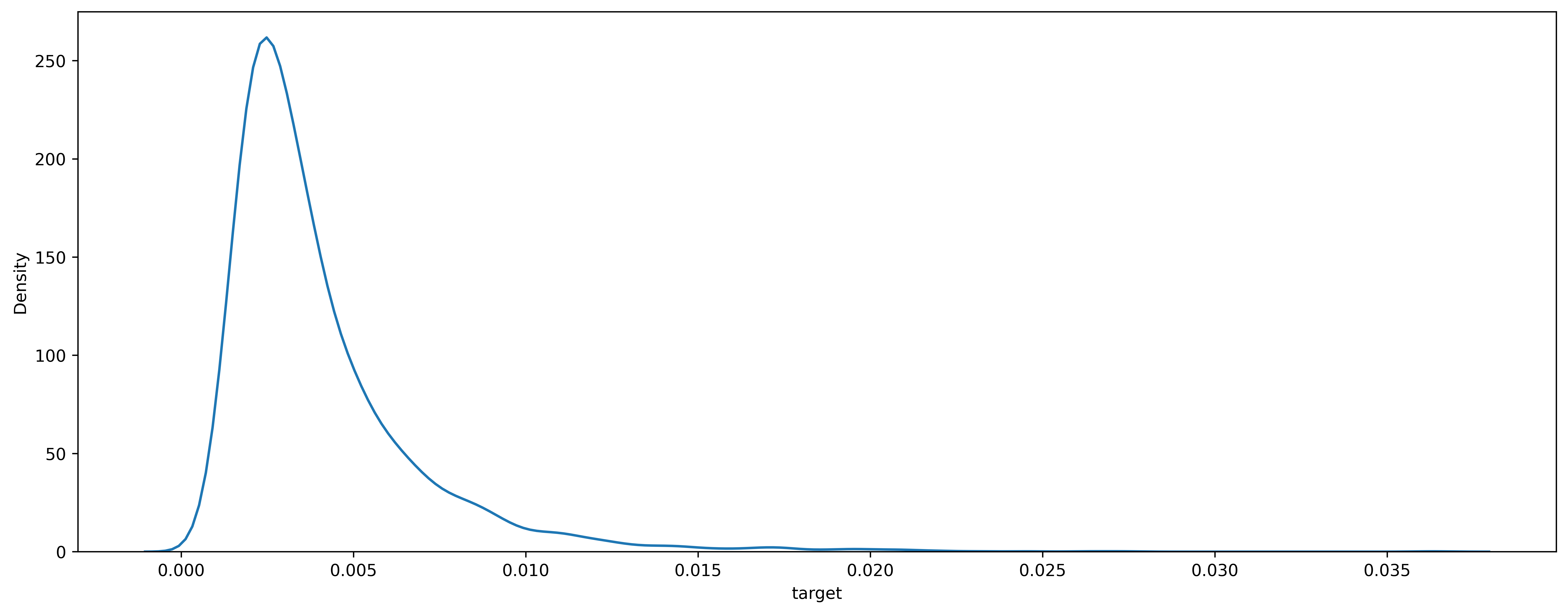
Empirical distribution of the realized volatility for a typical stock (the plot was generated using searborn’s utility kdeplot). Image by author.
Digression: benefits of fitting a probability distribution
It’s probably a good moment to address the question as to why we’d be interested in learning a probability distribution from the data instead of treating the realized volatility forecast as a regression problem (i.e. just trying to predict a number). In my opinion, the main motivations in this case are noise reduction and hedging against uncertainty.
As for the first one, it is well known that financial signals tend to be noisy. Although there are many different techniques to deal with this difficulty, I like the probability model approach because it attempts to handle the noise by design. Typically, the available data will be more than enough to robustly fit the few parameters of an underlying probabilistic model (and by this I mean a parametric probability distribution which the data at least approximately follow) even under the presence of noise. Moreover, you will automatically have at your disposal not just a number but a complete scenario with the probability of each event to help making optimal decisions. If I had to invest real money based on predictions, I would feel much more comfortable using a reasonably accurate probabilistic model that allows to quantify the risk rather than a black-box model that just outputs the next return, even at the cost of some precision loss.
However, all this comes with the rather heavy assumption that the data under analysis follows a parametric probability distribution. Is it the case in our problem? Well, I just started checking all known continuous probability distributions until I stumbled upon the inverse Gamma, which looked promising. I gave it a shot using the scipy.stats library and this is what happened.
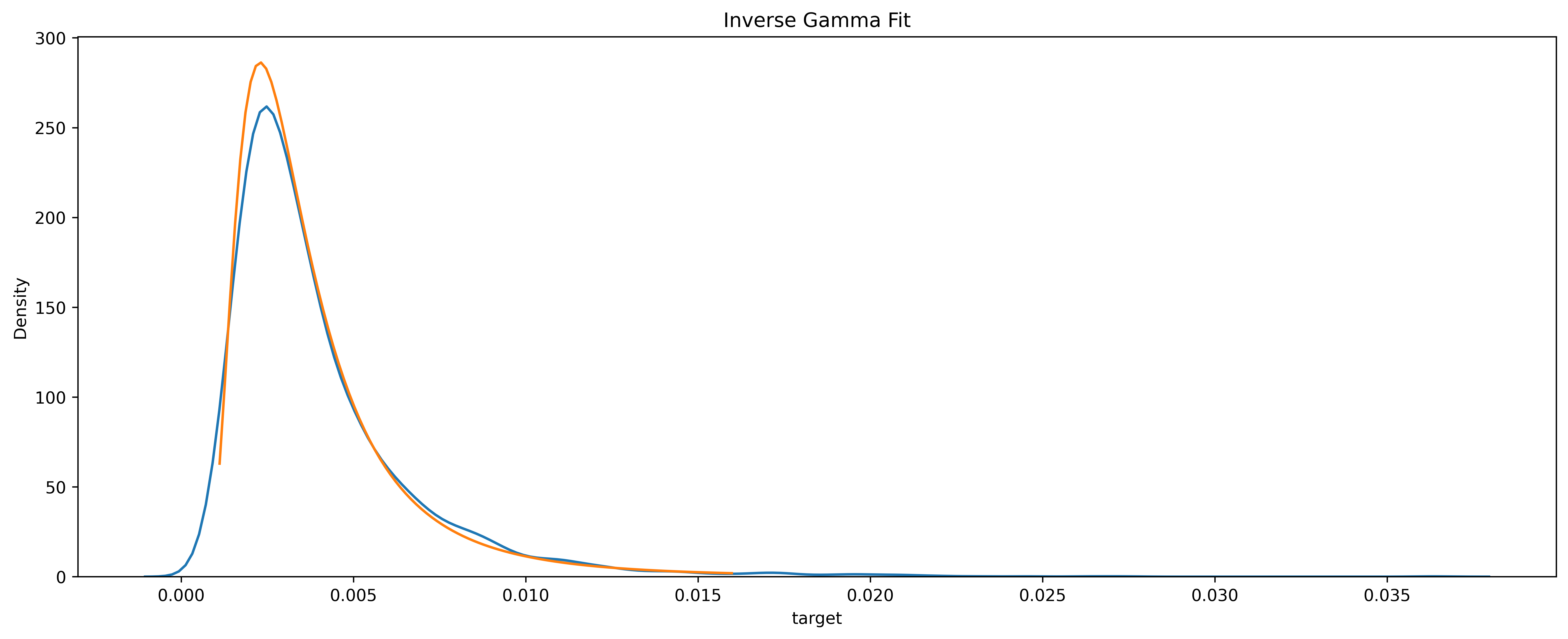
Fitting of the realized volatility with an inverse Gamma (empirical distribution in blue, fit in orange). Image by author.
Note: There is likely some firm theoretical foundation for choosing the inverse Gamma, related to it being the conjugate prior for the normal distribution (with known mean) in Bayesian analysis. But honestly I’m not sure… If you have a good explanation, please let me know!
Maximum likelihood estimation revisited
In simple probabilistic terms, regression algorithms in supervised learning attempt to learn some aspect of the distribution of a target variable \(y\) conditioned on data \(x\). Their training phase selects the best values for its parameters \(\theta\) (for instance, in a neural network \(\theta\) would be all the weights and biases of the neurons) in such a way that they minimize certain loss function computed on the training samples. To make a concrete example, if the loss function is the sum-of-squares error, the loss function \(L(\theta)\) is simply
\[L(\theta) := \sum_{i=1}^{n} (f(x_i;\theta) - y_i)^{2},\]where \(x_1, \cdots, x_n\) are the training samples with its corresponding labels \(y_1, \dots, y_n\) and \(f(x_i; \theta)\) is the guess of the model for the given parameters. It is well known that in this case, the model will try to approximate \(\mathbb{E}[y \vert x]\).
Back to the realized volatility problem, we have a reasonable hope that the volatility \(y\) conditioned on the data \(x\) follows an inverse Gamma distribution. Hence, by modifying the loss function we could try to have, say, a neural network learn the parameters of this distribution. As a result, we would obtain not only a decent approximation of \(\mathbb{E}[y \vert x]\), but we would actually know \(p(y \vert x)\)!
To be more precise, our hypothesis is that \(y \vert x\) follows a distribution that only depends on certain parameters \(\lambda\) which in turn depend on \(x\). The neural network will be used to learn the dependency of \(\lambda\) on \(x\). And what about the loss function? Well, you guessed it: we will try to maximize the likelihood, or equivalently, minimize minus the logarithm of the likelihood. So, in essence, this approach is nothing else than maximum likelihood on steroids.
Remark: More generally, what would happen if there was no evident probabilistic model for \(y \vert x\)? Bishop’s beautiful idea (link to the original paper) to overcome this shortcoming was to propose a mixture of gaussians. In principle, by adding enough gaussians, this parametric model is able to approximate any smooth density function arbitrarily well.
Coda
You can check the implementation details at my Github, but the credit really goes to this repo. I merely adapted the Mixture Density Layer from there to fit an inverse Gamma rather than a mixture of gaussians.
I would like to close this note by explaining how to choose our predictions once the distribution of \(y \vert x\) is fitted. The competition requires us to submit predictions \(\hat{y}\) in such a way that \(\mathbb{E} \left[ \left(\frac{y - \hat{y}}{y} \right)^2 \bigg \vert x \right]\) is minimized. By optimizing the expression for \(\hat{y}\), it is easy to find that the optimum value is \(\frac{\mathbb{E}\left[ \frac{1}{y} \bigg \vert x \right]}{\mathbb{E}\left[ \frac{1}{y^2} \bigg \vert x\right]}\). Notice just how hard and unstable would be to estimate these quantities without a probabilistic model, while a bit of pen and paper computations reveals that
\[\mathbb{E}\left[\frac{1}{y} \bigg \vert x \right] = \frac{\alpha}{\beta} \text{, } \mathbb{E}\left[\frac{1}{y^{2}} \bigg \vert x \right] = \frac{\alpha (\alpha+1)}{\beta}\]if \(y\vert x \sim \text{Inv-Gamma}(\alpha, \beta)\).